=======
![]()
Authors: Nicola Puletti, Gianluigi mazza
License: GPL3
AgeBandDecomposition provides tools for tree-ring
standardization based on the Age Band Decomposition (ABD) method, for
tree ring width standardization.
Install the stable version from CRAN:
install.packages("AgeBandDecomposition")or the development version from this GitLab page:
# install.packages("devtools")
remotes::install_git("https://gitlab.com/Puletti/agebanddecomposition_rpackage")
The package AgeBandDecomposition includes an example
dataset of 21 tree-ring width series of silver fir (Abies alba
Mill.) spanning from 1830 to 2021 and located in the Italian Apennine
core range (~ 1450 m a.s.l.), in the cool and moist oromediterranean
belt with optimal growing conditions for the species.
This example starts with downloading the files named “TRW_example.rwl” and “pith.offset.txt”, from the GitLab page of the package (see the folder “/main/studio/dati/”). For semplicity copy and paste these lines:
# Download example files from the package's GitLab page
package_gitlab_site <- 'https://gitlab.com/Puletti/agebanddecomposition_rpackage'
rwl_url <- "/-/raw/main/studio/dati/TRW_example.rwl"
po_url <- "/-/raw/main/studio/dati/pith.offset.txt"

# Create temporary files
tmpfile_rwl <- tempfile(fileext = ".rwl")
tmpfile_po <- tempfile(fileext = ".txt")

# Download the files
download.file(paste0(package_gitlab_site, rwl_url),
              tmpfile_rwl,
              mode = "wb")

download.file(paste0(package_gitlab_site, po_url),
              tmpfile_po,
              mode = "wb")

# Import the data
inData <- import_rwl(rwl_path = tmpfile_rwl,
                             po_path = tmpfile_po,
                             ageBands = '1010',
                             first_age_class = NULL,
                             zero_as_na = TRUE,
                             verbose = TRUE)

# View the result
inData
The object inData can be initially used to plot the mean
chronologies of raw tree-ring widths (mm) and raw basal area increments
(cm²), including their standard errors, alongside the corresponding
number of trees, using the two following functions:
plotTRW(inData)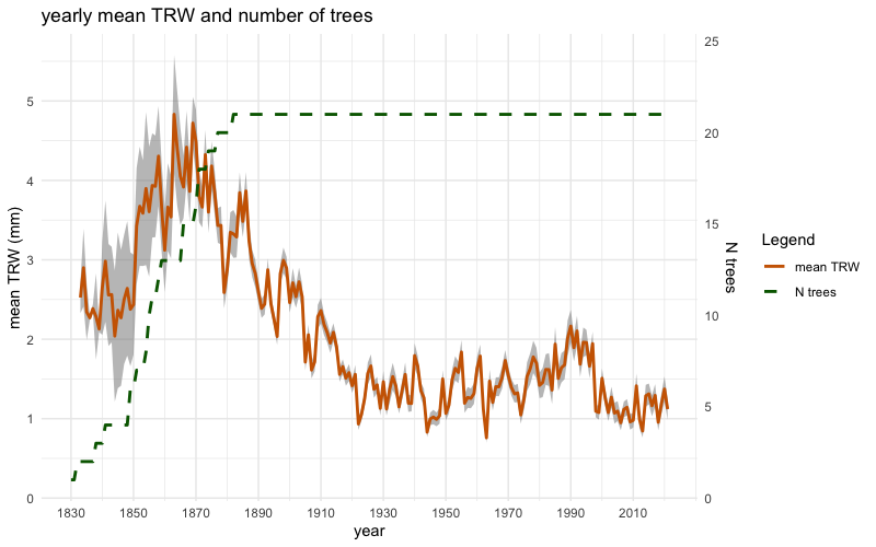
and
plotBAI(inData)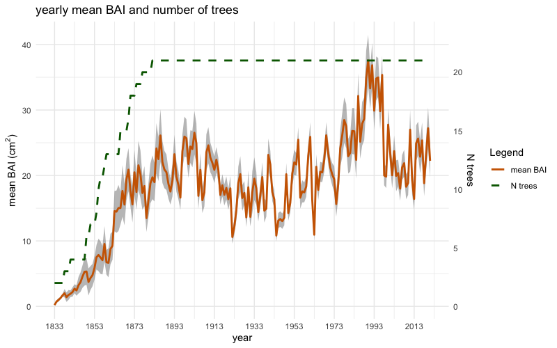
Tree-ring width values can be standardized using the
stdTRW() function, which removes the influences of local
site characteristics by dividing each tree-ring width by the mean width
of that series. This function is useful for exploratory analysis or
custom workflows:
# Optional: explore standardized TRW values
stdTRW_df <- stdTRW(inData[[1]])

# Calculate yearly averaged standardized TRW values
stdTRW_summary <- stdTRW_df |>
  dplyr::group_by(year) |>
  dplyr::summarise(
    N_trees = dplyr::n(),
    mean_stdTRW = mean(stdTRW, na.rm = TRUE)
  )
Note: The ABD() function (see below)
performs standardization internally, so this step is not required for
the ABD decomposition workflow.
The core function ABD() performs the Age Band
Decomposition analysis, which removes age-related growth trends to
isolate climate signals.
# ABD uses inData directly (standardization is done internally)
ABD_result <- ABD(inData, min_nTrees_year = 1)
# Export as .csv file
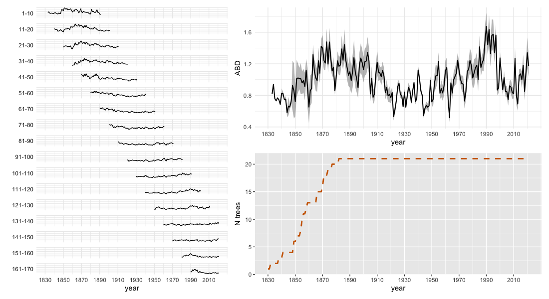
write.csv(ABD_result, file = 'your/path/file.csv')The plotABD() function provides a comprehensive
visualization of the results:
# Perform ABD analysis and visualize results
plotABD(inData, min_nTrees_year = 1)
The resulting multi-panel plot displays:
Left panel: Standardized tree-ring widths grouped by age bands (e.g., 1-10, 11-20, 21-30 years)
Top-right panel: Final ABD chronology with standard error bands, representing growth corrected for age effects
Bottom-right panel: Number of trees contributing to each year
Key parameters:
min_nTrees_year: Minimum number of trees required
per year within each age class (default: 3)
pct_stdTRW_th: Minimum proportion of data required
within an age band (default: 0.5 = 50%)
pct_Trees_th: Threshold for calculating mean values
(default: 0.3; increase to 0.5 for small samples <20 trees)