![]()
The FastJM package implements efficient computation of
semi-parametric joint model of longitudinal and competing risks data. To
view a brief guide on the purpose and use of this package, please refer
to our introductory
video.
jmcs)The FastJM package comes with several simulated
datasets. To fit a joint model, we use jmcs function. In
the example below, we are using the following built-in data sets:
require(FastJM)
require(survival)
data(ydata)
data(cdata)
fit <- jmcs(ydata = ydata, cdata = cdata,
            long.formula = response ~ time + gender + x1 + race,
            surv.formula = Surv(surv, failure_type) ~ x1 + gender + x2 + race,
            random =  ~ time| ID)
fit
#>
#> Call:
#>  jmcs(ydata = ydata, cdata = cdata, long.formula = response ~ time + gender + x1 + race, random = ~time | ID, surv.formula = Surv(surv, failure_type) ~ x1 + gender + x2 + race)
#>
#> Data Summary:
#> Number of observations: 3067
#> Number of groups: 1000
#>
#> Proportion of competing risks:
#> Risk 1 : 34.9 %
#> Risk 2 : 29.8 %
#>
#> Numerical intergration:
#> Method: pseudo-adaptive Guass-Hermite quadrature
#> Number of quadrature points:  6
#>
#> Model Type: joint modeling of longitudinal continuous and competing risks data
#>
#> Model summary:
#> Longitudinal process: linear mixed effects model
#> Event process: cause-specific Cox proportional hazard model with non-parametric baseline hazard
#>
#> Loglikelihood:  -8989.389
#>
#> Fixed effects in the longitudinal sub-model:  response ~ time + gender + x1 + race
#>
#>             Estimate      SE   Z value  p-val
#> (Intercept)  2.01853 0.05704  35.38803 0.0000
#> time         0.98292 0.03147  31.22885 0.0000
#> genderMale  -0.07766 0.05860  -1.32527 0.1851
#> x1          -1.47810 0.05851 -25.26356 0.0000
#> raceWhite    0.04527 0.05911   0.76581 0.4438
#>
#>         Estimate      SE  Z value  p-val
#> sigma^2  0.49182 0.01793 27.43751 0.0000
#>
#> Fixed effects in the survival sub-model:  Surv(surv, failure_type) ~ x1 + gender + x2 + race
#>
#>              Estimate      SE   Z value  p-val
#> x1_1          0.54672 0.18540   2.94892 0.0032
#> genderMale_1 -0.18781 0.11935  -1.57359 0.1156
#> x2_1         -1.10450 0.12731  -8.67602 0.0000
#> raceWhite_1  -0.10027 0.11802  -0.84960 0.3955
#> x1_2          0.62986 0.20064   3.13927 0.0017
#> genderMale_2  0.10834 0.13065   0.82926 0.4070
#> x2_2         -1.76738 0.15245 -11.59296 0.0000
#> raceWhite_2   0.03194 0.13049   0.24479 0.8066
#>
#> Association parameters:
#>               Estimate      SE Z value  p-val
#> (Intercept)_1  0.93973 0.12160 7.72809 0.0000
#> time_1         0.31691 0.19318 1.64051 0.1009
#> (Intercept)_2  0.96486 0.13646 7.07090 0.0000
#> time_2         0.03772 0.24137 0.15629 0.8758
#>
#>
#> Random effects:
#>   Formula: ~time | ID
#>                  Estimate      SE  Z value  p-val
#> (Intercept)       0.52981 0.03933 13.47048 0.0000
#> time              0.25885 0.02262 11.44217 0.0000
#> (Intercept):time -0.02765 0.02529 -1.09330 0.2743
The FastJM package can make dynamic prediction given the
longitudinal history information. Below is a toy example for competing
risks data. Conditional cumulative incidence probabilities for each
failure will be presented.
ND <- ydata[ydata$ID %in% c(419, 218), ]
ID <- unique(ND$ID)
NDc <- cdata[cdata$ID  %in% ID, ]
survfit <- survfitjmcs(fit,
                       ynewdata = ND,
                       cnewdata = NDc,
                       u = seq(3, 4.8, by = 0.2),
                       method = "GH",
                       obs.time = "time")
survfit
#>
#> Prediction of Conditional Probabilities of Event
#> based on the pseudo-adaptive Guass-Hermite quadrature rule with 6 quadrature points
#> $`218`
#>       times       CIF1      CIF2
#> 1  2.441634 0.00000000 0.0000000
#> 2  3.000000 0.09629588 0.1110072
#> 3  3.200000 0.11862304 0.1369133
#> 4  3.400000 0.15142590 0.1679708
#> 5  3.600000 0.18413127 0.1839693
#> 6  3.800000 0.21269800 0.2096528
#> 7  4.000000 0.23043413 0.2249182
#> 8  4.200000 0.25459317 0.2500146
#> 9  4.400000 0.25811390 0.2599361
#> 10 4.600000 0.28856883 0.2896654
#> 11 4.800000 0.30829095 0.3134531
#>
#> $`419`
#>       times       CIF1       CIF2
#> 1  2.432155 0.00000000 0.00000000
#> 2  3.000000 0.02972511 0.02073398
#> 3  3.200000 0.03757608 0.02601222
#> 4  3.400000 0.05003929 0.03270990
#> 5  3.600000 0.06332292 0.03635232
#> 6  3.800000 0.07563241 0.04273814
#> 7  4.000000 0.08376596 0.04677029
#> 8  4.200000 0.09564633 0.05378957
#> 9  4.400000 0.09743720 0.05674168
#> 10 4.600000 0.11449841 0.06602758
#> 11 4.800000 0.12639379 0.07432217
To assess the prediction accuracy of the fitted joint model, we may
run DynPredAccjmcs to assess the prediction accuracy by
calculating all available evaluation metrics.
res <- DynPredAccjmcs(
  object = fit,
  landmark.time = 3,
  horizon.time = c(3.6, 4, 4.4),
  obs.time = "time",
  method = "GH",
  maxiter = 1000,
  n.cv = 3,
  survinitial = TRUE,
  quantile.width = 0.25,
  metrics = c("AUC", "Cindex", "Brier", "MAE", "MAEQ")
)
#> The 1-th validation is done!
#> The 2-th validation is done!
#> The 3-th validation is done!

summary(res, metric = "Brier")
#>
#> Expected Brier Score at the landmark time of 3
#> based on 3 fold cross validation
#>   Horizon Time Brier Score 1 Brier Score 2
#> 1          3.6        0.0589        0.0348
#> 2          4.0        0.0889        0.0543
#> 3          4.4        0.1052        0.0687
summary(res, metric = "MAE")
#>
#> Expected mean absolute error at the landmark time of 3
#> based on 3 fold cross validation
#>   Horizon Time   MAE1   MAE2
#> 1          3.6 0.1188 0.0699
#> 2          4.0 0.1765 0.1085
#> 3          4.4 0.2090 0.1387
summary(res, metric = "MAEQ")
#>
#> Mean absolute error across quantiles of predicted risk scores at the landmark time of 3
#> based on 3 fold cross validation
#>   Horizon Time  MAEQ1  MAEQ2
#> 1          3.6 0.0208 0.0301
#> 2          4.0 0.0446 0.0403
#> 3          4.4 0.0477 0.0379
summary(res, metric = "AUC")
#>
#> Expected AUC at the landmark time of 3
#> based on 3 fold cross validation
#>   Horizon Time   AUC1   AUC2
#> 1          3.6 0.7367 0.7097
#> 2          4.0 0.7155 0.6760
#> 3          4.4 0.7337 0.7255
summary(res, metric = "Cindex")
#>
#> Expected Cindex at the landmark time of 3
#> based on 3 fold cross validation
#>   Horizon Time Cindex1 Cindex2
#> 1          3.6  0.6864  0.6773
#> 2          4.0  0.6860  0.6765
#> 3          4.4  0.6862  0.6758
Or we can calculate the overall, time-independent Cindex over the entire time period, evaluated by the linear predictor of the (cause-specific) Cox model.
Concord <- Concordancejmcs(seed = 100, fit, n.cv = 3)
#> The 1 th validation is done!
#> The 2 th validation is done!
#> The 3 th validation is done!
summary(Concord)
#>   Concordance1 Concordance2
#> 1 0.6721619 0.7037879mvjmcs)To fit a joint model with multiple longitudinal outcomes and
competing risks, we can use the mvjmcs function. In the
example below, we are using the following built-in data sets:
data(mvydata)
data(mvcdata)
library(FastJM)
mvfit <- mvjmcs(ydata = mvydata, cdata = mvcdata,
              long.formula = list(Y1 ~ X11 + X12 + time,
                                  Y2 ~ X11 + X12 + time),
              random = list(~ time | ID,
                            ~ 1 | ID),
              surv.formula = Surv(survtime, cmprsk) ~ X21 + X22,
              maxiter = 1000, opt = "optim",
              tol = 1e-3, print.para = FALSE)
#> runtime is:
#> Time difference of 57.60288 secs
mvfit
#>
#> Call:
#>  mvjmcs(ydata = mvydata, cdata = mvcdata, long.formula = list(Y1 ~ X11 + X12 + time, Y2 ~ X11 + X12 + time), random = list(~time | ID, ~1 | ID), surv.formula = Surv(survtime, cmprsk) ~ X21 + X22, maxiter = 1000, opt = "optim", tol = 0.001, print.para = FALSE)
#>
#> Data Summary:
#> Number of observations: 5645
#> Number of groups: 800
#>
#> Proportion of competing risks:
#> Risk 1 : 41.62 %
#> Risk 2 : 11.25 %
#>
#> Model Type: joint modeling of multivariate longitudinal continuous and competing risks data
#>
#> Model summary:
#> Longitudinal process: linear mixed effects model
#> Event process: cause-specific Cox proportional hazard model with non-parametric baseline hazard
#>
#> Fixed effects in the longitudinal sub-model:  list(Y1 ~ X11 + X12 + time, Y2 ~ X11 + X12 + time)
#>
#>                  Estimate      SE   Z value  p-val
#> (Intercept)_bio1  4.97406 0.05388  92.32120 0.0000
#> X11_bio1          1.46539 0.08053  18.19764 0.0000
#> X12_bio1          1.99793 0.01429 139.79571 0.0000
#> time_bio1         0.84275 0.03946  21.35698 0.0000
#> (Intercept)_bio2  9.97547 0.04927 202.44649 0.0000
#> X11_bio2          0.97966 0.07331  13.36293 0.0000
#> X12_bio2          2.00955 0.01309 153.48364 0.0000
#> time_bio2         0.99380 0.00455 218.63164 0.0000
#>
#>              Estimate      SE    Z value  p-val
#> sigma^2_bio1  0.49304 0.00018 2734.36540 0.0000
#> sigma^2_bio2  0.49758 0.00965   51.55778 0.0000
#>
#> Fixed effects in the survival sub-model:  Surv(survtime, cmprsk) ~ X21 + X22
#>
#>       Estimate      SE  Z value  p-val
#> X21_1  0.93618 0.13480  6.94491 0.0000
#> X22_1  0.51147 0.03167 16.15030 0.0000
#> X21_2 -0.21683 0.24922 -0.87006 0.3843
#> X22_2  0.48481 0.05923  8.18515 0.0000
#>
#> Association parameters:
#>                   Estimate      SE  Z value  p-val
#> (Intercept)_1bio1  0.49981 0.07535  6.63293 0.0000
#> time_1bio1         0.70822 0.08502  8.32969 0.0000
#> (Intercept)_1bio2 -0.54676 0.07972 -6.85843 0.0000
#> (Intercept)_2bio1  0.63217 0.13344  4.73764 0.0000
#> time_2bio1         0.66226 0.16726  3.95956 0.0001
#> (Intercept)_2bio2 -0.48377 0.15879 -3.04662 0.0023
#>
#>
#> Random effects:
#>   bio 1 :  ~time | ID
#>   bio 2 :  ~1 | ID
#>                       Estimate      SE  Z value  p-val
#> Intercept1             1.02117 0.06469 15.78498 0.0000
#> time1                  0.91580 0.05834 15.69838 0.0000
#> Intercept2             0.88206 0.05325 16.56574 0.0000
#> Intercept1:time1      -0.09307 0.04532 -2.05384 0.0400
#> Intercept1:Intercept2  0.04354 0.04052  1.07457 0.2826
#> time1:Intercept2      -0.06569 0.04224 -1.55510 0.1199
We can extract the components of the model as follows:
# Longitudinal fixed effects
fixef(mvfit, process = "Longitudinal")
#> (Intercept)_bio1         X11_bio1         X12_bio1        time_bio1 (Intercept)_bio2         X11_bio2         X12_bio2
#>        4.9740592        1.4653916        1.9979294        0.8427526        9.9754651        0.9796637        2.0095547
#>        time_bio2
#>        0.9937970
summary(mvfit, process = "Longitudinal")
#>        Longitudinal   coef     SE 95%Lower 95%Upper p-values
#> 1  (Intercept)_bio1 4.9741 0.0539   4.8685   5.0797        0
#> 2          X11_bio1 1.4654 0.0805   1.3076   1.6232        0
#> 3          X12_bio1 1.9979 0.0143   1.9699   2.0259        0
#> 4         time_bio1 0.8428 0.0395   0.7654   0.9201        0
#> 5  (Intercept)_bio2 9.9755 0.0493   9.8789  10.0720        0
#> 6          X11_bio2 0.9797 0.0733   0.8360   1.1234        0
#> 7          X12_bio2 2.0096 0.0131   1.9839   2.0352        0
#> 8         time_bio2 0.9938 0.0045   0.9849   1.0027        0
#> 9      sigma^2_bio1 0.4930 0.0002   0.4927   0.4934        0
#> 10     sigma^2_bio2 0.4976 0.0097   0.4787   0.5165        0

# Survival fixed effects
fixef(mvfit, process = "Event")
#> $Risk1
#>     X21_1     X22_1
#> 0.9361783 0.5114748
#>
#> $Risk2
#>      X21_2      X22_2
#> -0.2168317  0.4848128
summary(mvfit, process = "Event")
#>             Survival    coef exp(coef) SE(coef) 95%Lower 95%Upper 95%exp(Lower) 95%exp(Upper) p-values
#> 1              X21_1  0.9362    2.5502   0.1348   0.6720   1.2004        1.9581        3.3214   0.0000
#> 2              X22_1  0.5115    1.6677   0.0317   0.4494   0.5735        1.5674        1.7746   0.0000
#> 3              X21_2 -0.2168    0.8051   0.2492  -0.7053   0.2716        0.4940        1.3121   0.3843
#> 4              X22_2  0.4848    1.6239   0.0592   0.3687   0.6009        1.4459        1.8238   0.0000
#> 5  (Intercept)_1bio1  0.4998    1.6484   0.0754   0.3521   0.6475        1.4221        1.9108   0.0000
#> 6         time_1bio1  0.7082    2.0304   0.0850   0.5416   0.8749        1.7187        2.3986   0.0000
#> 7  (Intercept)_1bio2 -0.5468    0.5788   0.0797  -0.7030  -0.3905        0.4951        0.6767   0.0000
#> 8  (Intercept)_2bio1  0.6322    1.8817   0.1334   0.3706   0.8937        1.4487        2.4442   0.0000
#> 9         time_2bio1  0.6623    1.9392   0.1673   0.3344   0.9901        1.3972        2.6915   0.0001
#> 10 (Intercept)_2bio2 -0.4838    0.6165   0.1588  -0.7950  -0.1725        0.4516        0.8415   0.0023

# Random effects for first few subjects
head(ranef(mvfit))
#>   (Intercept)_bio1  time_bio1 (Intercept)_bio2
#> 1        1.2401906 -0.5307380      -1.20266480
#> 2       -0.5271435 -0.3345339       1.56044174
#> 3       -1.1560670  0.3260969       0.17152013
#> 4       -1.4226064 -1.9399773      -0.09515163
#> 5        0.2392488 -1.9542406       0.02231513
#> 6       -0.1187828 -0.0254132       0.06451794
The FastJM package can now make dynamic prediction in
the presence of multiple longitudinal outcomes. Below is a toy example
for competing risks data. Conditional cumulative incidence probabilities
for each failure will be presented.
require(dplyr)
#> Loading required package: dplyr
#>
#> Attaching package: 'dplyr'
#> The following object is masked from 'package:MASS':
#>
#>     select
#> The following objects are masked from 'package:stats':
#>
#>     filter, lag
#> The following objects are masked from 'package:base':
#>
#>     intersect, setdiff, setequal, union
set.seed(08252025)
sampleID <- sample(mvcdata$ID, 5, replace = FALSE)

subcdata <- mvcdata %>%
  dplyr::filter(ID %in% sampleID)

subydata <- mvydata %>%
  dplyr::filter(ID %in% sampleID)

### Set up a landmark time of 4.75 and make predictions at time u
survmvfit <- survfitmvjmcs(mvfit, seed = 100, ynewdata = subydata, cnewdata = subcdata,
                         u = c(7, 8, 9), Last.time = 4.75, obs.time = "time")

survmvfit
#>
#> Prediction of Conditional Probabilities of Event
#> based on the first order approximation
#> $`177`
#>   times       CIF1        CIF2
#> 1  4.75 0.00000000 0.000000000
#> 2  7.00 0.01835440 0.003145087
#> 3  8.00 0.02632333 0.004747017
#> 4  9.00 0.02939841 0.005963632
#>
#> $`182`
#>   times      CIF1       CIF2
#> 1  4.75 0.0000000 0.00000000
#> 2  7.00 0.2463582 0.03393494
#> 3  8.00 0.3325719 0.04805378
#> 4  9.00 0.3630881 0.05807832
#>
#> $`260`
#>   times       CIF1       CIF2
#> 1  4.75 0.00000000 0.00000000
#> 2  7.00 0.03315209 0.01750073
#> 3  8.00 0.04724973 0.02623700
#> 4  9.00 0.05262962 0.03281393
#>
#> $`305`
#>   times       CIF1       CIF2
#> 1  4.75 0.00000000 0.00000000
#> 2  7.00 0.02876153 0.01545058
#> 3  8.00 0.04104952 0.02319795
#> 4  9.00 0.04574922 0.02904055
#>
#> $`800`
#>   times       CIF1        CIF2
#> 1  4.75 0.00000000 0.000000000
#> 2  7.00 0.01293233 0.002102670
#> 3  8.00 0.01857301 0.003178285
#> 4 9.00 0.02075384 0.003996402JMMLSM)data(ydatah)
data(cdatah)
## fit a joint model
fit <- JMMLSM(cdata = cdatah, ydata = ydatah,
long.formula = Y ~ Z1 + Z2 + Z3 + time,
surv.formula = Surv(survtime, cmprsk) ~ var1 + var2 + var3,
variance.formula = ~ Z1 + Z2 + Z3 + time,
quadpoint = 6, random = ~ 1|ID, print.para = FALSE)
fit
#>
#> Call:
#> JMMLSM(cdata = cdatah, ydata = ydatah, long.formula = Y ~ Z1 + Z2 + Z3 + time, surv.formula = Surv(survtime, cmprsk) ~ var1 + var2 + var3, variance.formula = ~Z1 + Z2 + Z3 + time, random = ~1 | ID, quadpoint = 6, print.para = FALSE)
#>
#> Data Summary:
#> Number of observations: 1353
#> Number of groups: 200
#>
#> Proportion of competing risks:
#> Risk 1 : 45.5 %
#> Risk 2 : 32.5 %
#>
#> Numerical intergration:
#> Method: adaptive Guass-Hermite quadrature
#> Number of quadrature points: 6
#>
#> Model Type: joint modeling of longitudinal continuous and competing risks data with the presence of intra-individual variability
#>
#> Model summary:
#> Longitudinal process: Mixed effects location scale model
#> Event process: cause-specific Cox proportional hazard model with non-parametric baseline hazard
#>
#> Loglikelihood: -3621.603
#>
#> Fixed effects in mean of longitudinal submodel: Y ~ Z1 + Z2 + Z3 + time
#>
#> Estimate SE Z value p-val
#> (Intercept) 4.85342 0.12451 38.97918 0.0000
#> Z1 1.55235 0.16535 9.38841 0.0000
#> Z2 1.93774 0.14598 13.27409 0.0000
#> Z3 1.09289 0.05321 20.53796 0.0000
#> time 4.01129 0.02978 134.71376 0.0000
#>
#> Fixed effects in variance of longitudinal submodel: log(sigma^2) ~ Z1 + Z2 + Z3 + time
#>
#> Estimate SE Z value p-val
#> (Intercept) 0.50745 0.12838 3.95260 0.0001
#> Z1 0.50509 0.16005 3.15590 0.0016
#> Z2 -0.42508 0.13781 -3.08463 0.0020
#> Z3 0.14405 0.04494 3.20563 0.0013
#> time 0.09050 0.02422 3.73720 0.0002
#>
#> Survival sub-model fixed effects: Surv(survtime, cmprsk) ~ var1 + var2 + var3
#>
#> Estimate SE Z value p-val
#> var1_1 1.09710 0.32647 3.36051 0.0008
#> var2_1 0.19237 0.26154 0.73553 0.4620
#> var3_1 0.49611 0.08908 5.56951 0.0000
#>
#> var1_2 -0.88311 0.33702 -2.62037 0.0088
#> var2_2 0.80905 0.30127 2.68549 0.0072
#> var3_2 0.20871 0.09312 2.24143 0.0250
#>
#> Association parameters:
#> Estimate SE Z value p-val
#> (Intercept)_1 0.97480 0.62808 1.55202 0.1207
#> (Intercept)_2 -0.18580 0.47949 -0.38750 0.6984
#> var_(Intercept)_1 0.50030 0.58190 0.85977 0.3899
#> var_(Intercept)_2 -0.84481 0.52520 -1.60857 0.1077
#>
#>
#> Random effects:
#> Formula: ~1 | ID
#> Estimate SE Z value p-val
#> (Intercept) 0.49542 0.11339 4.36913 0.0000
#> var_(Intercept) 0.45581 0.11129 4.09578 0.0000
#> (Intercept):var_(Intercept) 0.26738 0.07854 3.40429 0.0007cnewdata <- cdatah[cdatah$ID %in% c(122, 152), ]
ynewdata <- ydatah[ydatah$ID %in% c(122, 152), ]
survfit <- survfitJMMLSM(fit, seed = 100, ynewdata = ynewdata, cnewdata = cnewdata,
u = seq(5.2, 7.2, by = 0.5), Last.time = "survtime",
obs.time = "time", method = "GH")
survfit
#>
#> Prediction of Conditional Probabilities of Event
#> based on the adaptive Guass-Hermite quadrature rule with 6 quadrature points
#> $`122`
#> times CIF1 CIF2
#> 1 5.069089 0.00000000 0.0000000
#> 2 5.200000 0.05596021 0.0000000
#> 3 5.700000 0.14584944 0.0000000
#> 4 6.200000 0.33882152 0.0000000
#> 5 6.700000 0.33882152 0.0000000
#> 6 7.200000 0.33882152 0.2171424
#>
#> $`152`
#> times CIF1 CIF2
#> 1 5.133665 0.0000000 0.00000000
#> 2 5.200000 0.0517717 0.00000000
#> 3 5.700000 0.1357406 0.00000000
#> 4 6.200000 0.3195265 0.00000000
#> 5 6.700000 0.3195265 0.00000000
#> 6 7.200000 0.3195265 0.06007945
oldpar <- par(mfrow = c(2, 2), mar = c(5, 4, 4, 4))
plot(survfit, include.y = TRUE)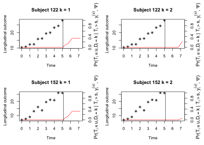
par(oldpar)If we assess the prediction accuracy of the fitted joint model using
Brier score as a calibration measure, we may run PEJMMLSM
to calculate the Brier score.
PE <- PEJMMLSM(fit, seed = 100, landmark.time = 3, horizon.time = c(4:6),
               obs.time = "time", method = "GH",
               n.cv = 3)
#> The 1 th validation is done!
#> The 2 th validation is done!
#> The 3 th validation is done!
summary(PE, error = "Brier")
#>
#> Expected Brier Score at the landmark time of 3
#> based on 3 fold cross validation
#>   Horizon Time Brier Score 1 Brier Score 2
#> 1            4    0.06369906    0.06194668
#> 2            5    0.10838731    0.11052099
#> 3            6    0.20187572    0.11613515
An alternative tool is to run MAEQJMMLSM to calculate
the prediction error by comparing the predicted and empirical risks
stratified on different risk groups based on quantile of the predicted
risks.
MAEQ <- MAEQJMMLSM(fit, seed = 100, landmark.time = 3,
                   horizon.time = c(4:6),
                   obs.time = "time", method = "GH", n.cv = 3)
#> The 1 th validation is done!
#> The 2 th validation is done!
#> The 3 th validation is done!
summary(MAEQ)
#>
#> Mean absolute error across quantile of predicted risk scores at the landmark time of 3
#> based on 3 fold cross validation
#>   Horizon Time  CIF1  CIF2
#> 1            4 0.096 0.066
#> 2            5 0.119 0.086
#> 3            6 0.114 0.107
Using area under the ROC curve (AUC) as a discrimination measure, we
may run AUCJMMLSM to calculate the AUC score.
AUC <- AUCJMMLSM(fit, seed = 100, landmark.time = 3, horizon.time = c(4:6),
                 obs.time = "time", method = "GH",
                 n.cv = 3, metric = "AUC")
#> The 1 th validation is done!
#> The 2 th validation is done!
#> The 3 th validation is done!
summary(AUC)
#>
#> Expected AUC at the landmark time of 3
#> based on 3 fold cross validation
#>   Horizon Time      AUC1      AUC2
#> 1            4 0.5502137 0.6839226
#> 2            5 0.6182312 0.6523506
#> 3            6 0.6103724 0.7065657
Alternatively, we can also calculate concordance index (Cindex) as another discrimination measure.
## evaluate prediction accuracy of fitted joint model using cross-validated mean Cindex
Cindex <- AUCJMMLSM(fit, seed = 100, landmark.time = 3, horizon.time = c(4:6),
                  obs.time = "time", method = "GH",
                  n.cv = 3, metric = "Cindex")
#> The 1 th validation is done!
#> The 2 th validation is done!
#> The 3 th validation is done!
summary(Cindex)
#>
#> Expected Cindex at the landmark time of 3
#> based on 3 fold cross validation
#>   Horizon Time   Cindex1   Cindex2
#> 1            4 0.6154102 0.6509733
#> 2            5 0.6132650 0.6463436
#> 3            6 0.6125965 0.6463436
Or we can calculate the overall, time-independent Cindex over the entire time period, evaluated by the linear predictor of the (cause-specific) Cox model.
Concord <- ConcordanceJMMLSM(seed = 100, fit, n.cv = 3)
#> The 1 th validation is done!
#> The 2 th validation is done!
#> The 3 th validation is done!
summary(Concord)
#>   Concordance1 Concordance2
#> 1 0.7943508 0.7413602In order to create simulated data for mvjmcs, we can use
the simmvJMdata function, which creates longitudinal and
survival data as a nested list (which are unpacked the this example).
When first calling the function, it provides censoring and risk
rates.
# Simulate data
  sim <- simmvJMdata(seed = 100, N = 50) # returns list of cdata and ydata for a sample size of 50
#> The censoring rate is: 44%
#> The risk 1 rate is: 48%
#> The risk 2 rate is: 8%
  c_data <- sim$mvcdata # survival-side data, one row per ID
  y_data <- sim$mvydata # longitudinal measurements (multiple rows per ID)
Below is the simulated longitudinal data for multiple biomarkers, wherein Y1 and Y2 represent our biomarkers and X11 and X12 represent measurement-level predictors for the longitudinal submodel.
head(y_data)
#>   ID time       Y1       Y2 X11       X12
#> 1  1  0.0 2.325975 3.493627   0 -2.347892
#> 2  1  0.7 2.328122 4.649502   0 -2.347892
#> 3  1  1.4 2.793674 6.112850   0 -2.347892
#> 4  1  2.1 2.221392 5.375753   0 -2.347892
#> 5  1  2.8 1.864348 4.481401   0 -2.347892
#> 6  1  3.5 3.988955 5.496069   0 -2.347892
Below is the simulated survival data wherein X21 and X22 represent patient-level predictors for the survival model.
head(c_data)
#>   ID   survtime cmprsk X21        X22
#> 1  1 6.10116281      0   0 -2.3478921
#> 2  2 0.05456028      1   1  0.1826885
#> 3  3 6.52978656      0   1  2.3791087
#> 4  4 0.04942950      1   1  2.7961091
#> 5  5 6.96785721      0   0 -3.8530560
#> 6  6 7.20378227      0   0  1.1237335